How Revenue Buildup is actually Forecasted?

Not one growth rate on a total — three product categories, three scenarios, and a formula that runs all the way to DCF.

Before a model can estimate profit, cash flow or valuation, it has to answer one question first: how much revenue will the company actually make?

A lazy answer applies a single growth rate to last year’s total and calls it a forecast. The GCPL model does something more useful — it builds revenue up from the company’s actual product categories, then stress-tests that forecast against three different futures.

What “Revenue Buildup” means

Revenue buildup means constructing a company’s total revenue from its underlying sources.

The basic idea is:

Revenue from Product Categories + Other Operating Revenue = Final Revenue

In our model, the major product categories are:

• Home Care
• Hair Care
• Personal Care

There is also a separate category called Other Operating Revenues.

This approach is useful because it allows us to understand where the company’s revenue comes from and apply assumptions to different components.

Nine years, two kinds of data

The Revenue Buildup sheet runs from 2019 to 2027. The first four years are actuals; everything from 2023 onward is estimated — marked A for Actual and E for Estimated.

Step 1: Revenue by product category

Three categories carry the business: Home Care, Hair Care and Personal Care. Here’s how each actually performed between 2019 and 2022:

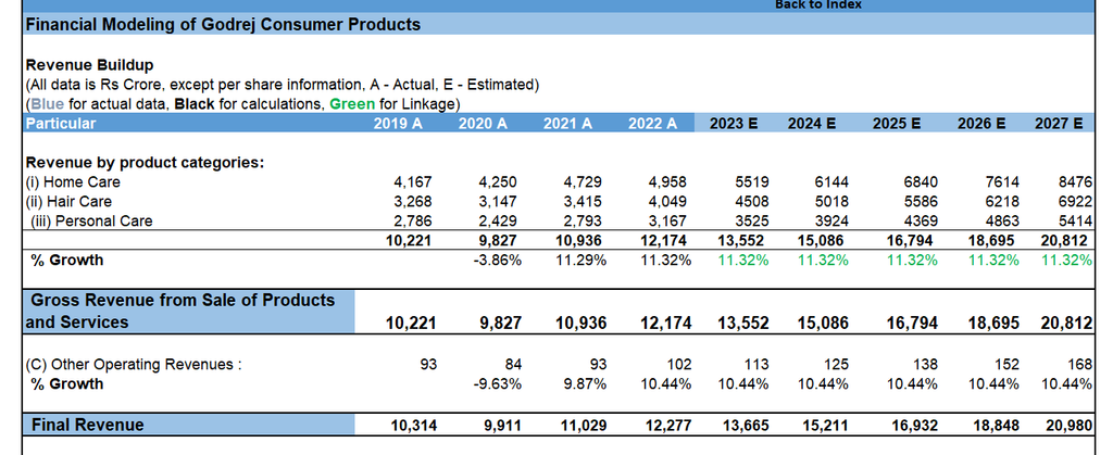
For every category, the estimated years use the same logic:

Step 2: Adding it up — and Checking the pace

Once each category is forecast, the model sums them into a total — never the other way around:

Build the total from its components, instead of forecasting the total independently. Change one category’s assumption and the total updates itself — nothing needs to be re-entered by hand.

The sheet also tracks how fast that total is growing:

Step 3-5: Gross Revenue

The combined product-category total is labelled Gross Revenue from Sale of Products and Services. Separately, the model tracks Other Operating Revenue — a smaller, non-product income line, forecast the same way (previous year × growth rate):

The two pieces then come together as Final Revenue — the number that actually flows into the Income Statement:

Three futures, not one

Nobody knows exactly what GCPL’s revenue will look like in 2027. So instead of pretending to, the model runs three scenarios side by side:

The point isn’t to guess which scenario wins. It’s to see how sensitive the whole model is to the growth assumption — which matters far more than most people expect once it reaches the valuation stage.

How a Scenario actually gets applied

The three growth rates don’t all run at once — a single selection, made on the DCF sheet, decides which one is live:

The Naive Way vs. The Buildup Way

Where Final Revenue actually goes

Key Takeaways

Start with the business
Know where revenue actually comes from before forecasting it.

Separate actual from estimated
History tells you what happened; assumptions decide what might.

Forecast components, not totals
Build revenue up from its underlying categories.

Use a consistent formula
Previous Year Revenue × (1 + Growth Rate), applied everywhere.

Run scenarios
Bullish, Normal and Bearish test how sensitive the model really is.

Link the schedules
Final Revenue should flow forward, not sit isolated in one tab.

Assumptions drive valuation
Every growth assumption here eventually reaches the DCF.

Read More: How to actually read a Financial Model